Specializing Python with E-graphs

We've explored progressively more sophisticated techniques for optimizing numerical computations. We started with basic MLIR concepts, moved through memory management and linear algebra, and then neural network implementations. Each layer has added new capabilities for expressing and optimizing computations. Now we're reading to build our first toy compiler for Python expressions.

In this section, we'll explore how to use the egglog library to perform term rewriting and optimization on Python expressions and compile them into MLIR.

The entire source code for this section is available on GitHub.

Equality Saturaiton and E-Graphs

Before we dive into the implementation, let's review the key concepts of equality saturation and e-graphs.

Take as an example if we have the rewrites.

x * 2 → x << 1
x*y/x → y

And we try to apply it over the expression (a * 2)/2 becomes (a << 1)/2. However we should have cancelled the 2 in the numerator and denominator and got a which results in a simpler expression. The order of rewrites is important and we want to find an optimal order of rewrites that reduces the expression to a form according to a cost function. This is called the phase ordering problem.

The egg library employs an approach that involves exhaustively applying all possible rewrites to an expression, effectively addressing the phase ordering problem through the use of an e-graph. This approach allows for the exploration of all possible rewrites, followed by the extraction of the most optimal form of the expression.

In linear algebra for example, matrix operations with NumPy like transpose, multiplication, are quite expensive because they involve touching every element of the matrix. But there is a wide range of identities that can be applied to reduce the number of operations.

Compilers like LLVM and even the linalg dialect of MLIR doesn't know about these identities and so can't necessarily abstract away the expensive operations by applying rewrites. However at a high-level (our core language) we can use e-graph to produce much more efficient tensor manipulation operations before lowering them into MLIR.

For example, the following identities are quite common in linear algebra:

(A B)^T = B^T A^T

(A^T)^T = A

Or in Python:

np.transpose(A * B) = np.transpose(B) * np.transpose(A)
np.transpose(np.transpose(A)) == A

By applying these rules, we can optimize NumPy expressions at compile time, leading to significant performance improvements. For instance, in our example, we've successfully reduced three loops—comprising one multiplication and two transposes—down to just two loops, which consist of one multiplication and one transpose. This optimization not only simplifies the computation but also enhances efficiency. In common uses of NumPy, there are numerous opportunities for such optimizations, often referred to as low-hanging fruit. These optimizations can be systematically applied to reduce the number of operations required, thereby streamlining the execution of numerical computations. This is particularly beneficial before even LLVM's auto-vectorization comes into play, as it allows us to leverage the full potential of our expressions and achieve faster execution times.

An e-graph (equality graph) is a data structure that compactly represents many equivalent expressions. Instead of maintaining a single canonical form for expressions, e-graphs maintain classes of equivalent expressions. This approach allows for more flexible and efficient term rewriting.

Let's look at a concrete example using egglog library to do basic simplification. First we have to define our expression model.

from __future__ import annotations
from egglog import *
 
class Num(Expr):
    def __init__(self, value: i64Like) -> None: ...
    
    @classmethod
    def var(cls, name: StringLike) -> Num: ...
    
    def __add__(self, other: Num) -> Num: ...
    
    def __mul__(self, other: Num) -> Num: ...
 
# Create an e-graph to store our expressions
egraph = EGraph()
 
# Define our expressions and give them names in the e-graph
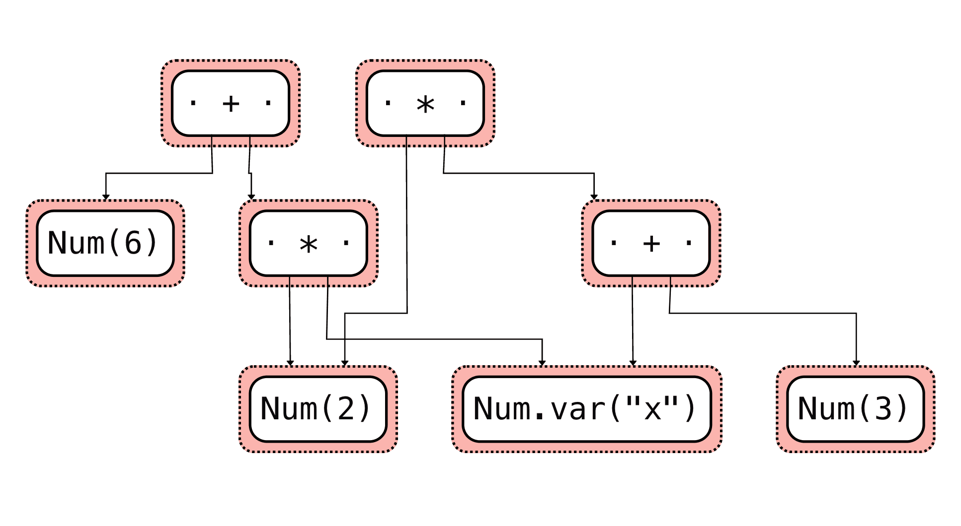
expr1 = egraph.let("expr1", Num(2) * (Num.var("x") + Num(3)))  # 2 * (x + 3)
expr2 = egraph.let("expr2", Num(6) + Num(2) * Num.var("x"))    # 6 + 2x
 
# Define our rewrite rules using a decorated function
@egraph.register
def _num_rule(a: Num, b: Num, c: Num, i: i64, j: i64):
    yield rewrite(a + b).to(b + a)                    # Commutativity of addition
    yield rewrite(a * (b + c)).to((a * b) + (a * c))  # Distributive property
    yield rewrite(Num(i) + Num(j)).to(Num(i + j))     # Constant folding for addition
    yield rewrite(Num(i) * Num(j)).to(Num(i * j))     # Constant folding for multiplication
 
# Apply rules until no new equalities are found
egraph.saturate()
 
# Check if expr1 and expr2 are equivalent
egraph.check(eq(expr1).to(expr2))
 
# Extract the simplified form of expr1
egraph.extract(expr1)

Using the egraph.display() function we can visualize the e-graph.

The input expression before equality saturation:

Then the output with all the equivalences classes is a network of expressions:

From there we can extract the expression we want according to a custom cost function.

Foundation Layer

Ok now let's apply this to our basic expression compiler. Our compiler pipeline has several key stages:

Python function decoration and type annotation
Expression tree extraction
Term rewriting and optimization using e-graphs
MLIR code generation
LLVM compilation and JIT execution

The foundation layer of our compiler provides the core abstractions for representing and manipulating mathematical expressions. This layer is crucial as it forms the basis for all higher-level optimizations and transformations. Let's explore each component in detail.

Expression Model (`expr_model.py`)

At the heart of our compiler is an expression model that represents mathematical expressions as an abstract syntax tree (AST). The model is implemented using Python's dataclasses for clean and efficient representation.

Core Expression Types

The base class for all expressions is the Expr class, which provides the fundamental operations:

@dataclass(frozen=True)
class Expr:
    def __add__(self, other: Expr) -> Expr:
        return Add(self, as_expr(other))
    
    def __mul__(self, other: Expr) -> Expr:
        return Mul(self, as_expr(other))
    # ... other operations

The expression model consists of three fundamental types:

Literals: Constants in our expressions

@dataclass(frozen=True)
class FloatLiteral(Expr):
    fval: float  # Floating-point constant
 
@dataclass(frozen=True)
class IntLiteral(Expr):
    ival: float  # Integer constant

Symbols: Variables and function names

@dataclass(frozen=True)
class Symbol(Expr):
       name: str  # Variable or function name

Operations: Both unary and binary operations

@dataclass(frozen=True)
class UnaryOp(Expr):
       operand: Expr  # Single operand
 
@dataclass(frozen=True)
class BinaryOp(Expr):
    lhs: Expr  # Left-hand side
    rhs: Expr  # Right-hand side

And then we can define instances of our operations.

@dataclass(frozen=True)
class Add(BinaryOp): pass      # Addition
...
 
@dataclass(frozen=True)
class Sin(UnaryOp): pass       # Sine

Built-in Functions (`builtin_functions.py`)

The built-in functions module provides a NumPy-like interface for mathematical operations. This makes it easier for users to write expressions in a familiar syntax while still leveraging our optimization framework. It includes common mathematical constants and helper functions for operations like absolute value.

# A mock NumPy namespace that we convert into our own expression model
 
import math
from mlir_egglog.expr_model import (
    sin,
    cos,
    tan,
    asin,
    acos,
    atan,
    tanh,
    sinh,
    cosh,
    sqrt,
    exp,
    log,
    log10,
    log2,
    float32,
    int64,
    maximum,
)  # noq
 
# Constants
e = math.e
pi = math.pi
 
 
# Define abs function
def abs(x):
    return maximum(x, -x)
 
 
def relu(x):
    return maximum(x, 0.0)
 
 
def sigmoid(x):
    return 1.0 / (1.0 + exp(-x))
 
 
__all__ = [
    "sin",
    "cos",
    "tan",
    "asin",
    "acos",
    "atan",
    "tanh",
    "sinh",
    "cosh",
    "sqrt",
    "exp",
    "log",
    "log10",
    "log2",
    "float32",
    "int64",
    "e",
    "pi",
    "maximum",
    "abs",
]

Term IR (`term_ir.py`)

The Term IR layer provides an intermediate representation optimized for term rewriting and equality saturation. A key feature of the Term IR is a cost model for different operations:

COST_BASIC_ARITH = 1   # Basic arithmetic (single CPU instruction)
COST_CAST = 2          # Type conversion operations
COST_DIV = 5           # Division
COST_POW_INTEGER = 10  # Integer power
COST_SQRT = 20         # Square root
COST_LOG = 30          # Logarithm
COST_EXP = 40          # Exponential
COST_POW = 50          # General power operation
COST_TRIG_BASIC = 75   # Basic trigonometric functions
COST_HYPERBOLIC = 180  # Hyperbolic functions

These costs are used by the e-graph optimization engine to make decisions about which transformations to apply. The costs roughly correspond to the computational complexity of each operation on modern hardware.

from __future__ import annotations
 
import egglog
from egglog import StringLike, i64, f64, i64Like, f64Like  # noqa: F401
from egglog import RewriteOrRule, rewrite
from typing import Generator
from mlir_egglog.expr_model import Expr, FloatLiteral, Symbol, IntLiteral
from abc import abstractmethod
 
def as_egraph(expr: Expr) -> Term:
    """
    Convert a syntax tree expression to an egraph term.
    """
    from mlir_egglog import expr_model
 
    match expr:
        # Literals and Symbols
        case FloatLiteral(fval=val):
            return Term.lit_f32(val)
        case IntLiteral(ival=val):
            return Term.lit_i64(int(val))
        case Symbol(name=name):
            return Term.var(name)
 
        # Binary Operations
        case expr_model.Add(lhs=lhs, rhs=rhs):
        
        # Rest of the operations
        ...

The cost model is used to guide the e-graph optimization engine to find the most cost-effective implementation according to our cost model. For example

e^x \cdot e^x \cdot e^x = e^{3x}

The LHS has 3 multiplications and the RHS has 1 multiplication. So the cost applied to the extraction will select the RHS.

Transformation Layer

One of the most powerful features of our compiler is its ability to symbolically interpret Python functions. This process transforms regular Python functions into our IR representation, allowing us to apply optimizations on the resulting expression tree.

The interpretation process is handled by the interpret function:

import types
import inspect
 
from mlir_egglog import expr_model as ir
 
 
def interpret(fn: types.FunctionType, globals: dict[str, object]):
    """
    Symbolically interpret a python function.
    """
    # Get the function's signature
    sig = inspect.signature(fn)
 
    # Create symbolic parameters for each of the function's arguments
    params = [n for n in sig.parameters]
    symbolic_params = [ir.Symbol(name=n) for n in params]
 
    # Bind the symbolic parameters to the function's arguments
    ba = sig.bind(*symbolic_params)
 
    # Inject our globals (i.e. np) into the function's globals
    custom_globals = fn.__globals__.copy()
    custom_globals.update(globals)
 
    # Create a temporary function with our custom globals
    tfn = types.FunctionType(
        fn.__code__,
        custom_globals,
        fn.__name__,
        fn.__defaults__,
        fn.__closure__,
    )
    return tfn(*ba.args, **ba.kwargs)

The function begins with parameter analysis, where it analyzes the input function's signature to determine its parameters. For each parameter, it creates a symbolic representation using our Symbol class. These symbols will be used to track variables through the expression tree.

Next, the symbolic parameters are bound to the function's argument slots, creating a mapping between parameter names and their symbolic representations. The function then injects our custom implementations of mathematical operations, such as NumPy functions, into the function's global namespace. This allows us to intercept calls to these functions and replace them with our symbolic operations.

A temporary function is created with the modified globals, while retaining the same code, name, and closure as the original function. Finally, the function is executed with the symbolic parameters, resulting in an expression tree that represents the computation.

For example, given a Python function:

def f(x, y):
    return np.sin(x) + np.cos(y)

The interpretation process will:

Create symbols for x and y
Replace np.sin and np.cos with our symbolic versions
Execute the function with symbolic inputs
Return an expression tree representing Sin(Symbol("x")) + Cos(Symbol("y"))

This symbolic interpretation is what allows us to capture Python computations in a form that can be optimized using our e-graph machinery.

IR Conversion (`ir_to_mlir.py`)

The IR to MLIR conversion layer serves as a crucial bridge between our high-level expression representation and MLIR's lower-level dialect. This conversion process is implemented in ir_to_mlir.py and involves several steps that leverage Python's dynamic execution capabilities along with AST manipulation.

The conversion pipeline begins with the convert_term_to_expr function, which transforms an IR term into our internal expression model. This function employs Python's built-in ast module to parse and manipulate the abstract syntax tree of the term. The process is particularly interesting because it uses Python's execution environment as part of the conversion process.

When a term arrives for conversion, it first goes through AST parsing. The function creates a Python AST from the string representation of the term, which allows us to manipulate the code structure before execution. A key part of this process is the mangle_assignment function, which ensures the result of the expression is properly captured in a variable named _out. This mangling step is crucial because it provides a way to extract the final result from the execution environment.

The execution environment is carefully constructed using a function_map dictionary that maps operation names to their corresponding implementations. This map includes basic arithmetic operations (Add, Sub, Mul, Div), mathematical functions (Sin, Cos, Exp, Log), and type conversion operations (CastF32, CastI64). Each of these operations is mapped to either a method from our expression model or a function from our builtin functions module.

The second major component is the convert_term_to_mlir function, which takes the converted expression and generates MLIR code. This function handles the final transformation into MLIR's textual format. It processes function arguments through the argspec parameter, creating a mapping between argument names and their MLIR representations (e.g., converting x to %arg_x). The actual MLIR generation is delegated to the MLIRGen class, which walks through the expression tree and produces corresponding MLIR operations.

For example, when converting a simple arithmetic expression like a + b * c, the pipeline would:

Parse the expression into an AST
Transform it into our internal expression model using the function map
Generate MLIR code with proper memory references and operations
Wrap the operations in a proper MLIR function structure with appropriate type annotations

def convert_term_to_expr(tree: IRTerm) -> ir.Expr:
    """
    Convert a term to an expression.
    """
 
    # Parse the term into an AST
    astree = ast.parse(str(tree))
 
    # Mangle the assignment
    astree.body[-1] = ast.fix_missing_locations(mangle_assignment(astree.body[-1]))  # type: ignore
 
    # Execute the AST
    globals: dict[str, Any] = {}
    exec(compile(astree, "<string>", "exec"), function_map, globals)
 
    # Get the result
    result = globals["_out"]
    return result
 
 
def convert_term_to_mlir(tree: IRTerm, argspec: str) -> str:
    """
    Convert a term to MLIR.
    """
 
    expr = convert_term_to_expr(tree)
    argnames = map(lambda x: x.strip(), argspec.split(","))
    argmap = {k: f"%arg_{k}" for k in argnames}
    source = MLIRGen(expr, argmap).generate()
    return source

Optimization Layer

Now we can start to write our own rewrite rules to apply over our expression tree.

The birewrite_subsume helper function is a generator that yields rewrite rules for the e-graph. It takes two terms and yields a rewrite rule that converts the first term to the second, making the first term unable to be matched against or extracted. We use this to unidirectionally convert generic Terms into specialized binary and unary operations.

def birewrite_subsume(a: Term, b: Term) -> Generator[RewriteOrRule, None, None]:
    yield rewrite(a, subsume=True).to(b)
    yield rewrite(b).to(a)

The basic simplification module implements fundamental mathematical rewrites that form the foundation of our term rewriting system. These rules are organized in the basic_math ruleset and include several key categories of transformations:

Term Translation Rules: These rules allow conversion between generic Terms and their specialized forms (Add, Mul, Div, Pow)
Identity Rules: Rules for handling mathematical identities like $x + 0 = x$ and $x \cdot 1 = x$
Associativity Rules: Rules that handle the associative properties of operations like $(x + y) + z = x + (y + z)$
Power Rules: Special handling for powers, including cases like $x^0 = 1$ and $x^1 = x$
Arithmetic Simplification: Rules that simplify common arithmetic patterns like $x + x = 2 \cdot x$

Each rule is implemented using egglog's rewrite system.

from mlir_egglog.term_ir import Term, Add, Mul, Div, Pow, PowConst, birewrite_subsume
from egglog import RewriteOrRule, ruleset, rewrite, i64, f64
from typing import Generator
 
 
@ruleset
def basic_math(
    x: Term, y: Term, z: Term, i: i64, f: f64
) -> Generator[RewriteOrRule, None, None]:
    # Allow us to translate Term into their specializations
    yield from birewrite_subsume(x + y, Add(x, y))
    yield from birewrite_subsume(x * y, Mul(x, y))
    yield from birewrite_subsume(x / y, Div(x, y))
    yield from birewrite_subsume(x**y, Pow(x, y))
 
    # x + 0 = x (integer case)
    yield rewrite(Add(x, Term.lit_i64(0))).to(x)
    # x + 0.0 = x (float case)
    yield rewrite(Add(x, Term.lit_f32(0.0))).to(x)
    # 0.0 + x = x (float case)
    yield rewrite(Add(Term.lit_f32(0.0), x)).to(x)
 
    # x * 1 = x
    yield rewrite(Mul(x, Term.lit_i64(1))).to(x)
 
    # x * 0 = 0
    yield rewrite(Mul(x, Term.lit_i64(0))).to(Term.lit_i64(0))
 
    # (x + y) + z = x + (y + z)
    yield rewrite(Add(x, Add(y, z))).to(Add(Add(x, y), z))
 
    # (x * y) * z = x * (y * z)
    yield rewrite(Mul(x, Mul(y, z))).to(Mul(Mul(x, y), z))
 
    # x + x = 2 * x
    yield rewrite(Add(x, x)).to(Mul(Term.lit_i64(2), x))
 
    # x * x = x^2
    yield rewrite(Mul(x, x)).to(Pow(x, Term.lit_i64(2)))
 
    # (x^y) * (x^z) = x^(y + z)
    yield rewrite(Pow(x, y) * Pow(x, z)).to(Pow(x, Add(y, z)))
 
    # x^i = x * x^(i - 1)
    yield rewrite(Pow(x, Term.lit_i64(i))).to(PowConst(x, i))
 
    # x^0 = 1
    yield rewrite(PowConst(x, 0)).to(Term.lit_f32(1.0))
 
    # x^1 = x
    yield rewrite(PowConst(x, 1)).to(x)
 
    # x^i = x * x^(i - 1)
    yield rewrite(PowConst(x, i)).to(Mul(x, PowConst(x, i - 1)), i > 1)

Similar to the basic simplification module, the trigonometric simplification module provides a comprehensive set of rules for simplifying expressions involving trigonometric and hyperbolic functions. The trig_simplify ruleset implements several important categories of transformations:

Fundamental Identities: Core trigonometric identities like $\sin^2(x) + \cos^2(x) = 1$
Double Angle Formulas: Rules for simplifying expressions like $\sin(x + y)$ and $\cos(x + y)$
Hyperbolic Identities: Similar rules for hyperbolic functions, including identities for $\sinh$ , $\cosh$ , and $\tanh$

These rules are particularly important for optimizing numerical computations involving trigonometric functions, which are common in scientific computing and machine learning applications. The module carefully balances the tradeoff between expression simplification and computational efficiency, using the cost model defined in the Term IR to guide its decisions.

from mlir_egglog.term_ir import Sin, Cos, Sinh, Cosh, Tanh, Term, Pow, Add
from egglog import ruleset, i64, f64
from egglog import rewrite
 
 
@ruleset
def trig_simplify(x: Term, y: Term, z: Term, i: i64, fval: f64):
    # Fundamental trig identities
    # sin²(x) + cos²(x) = 1
    two = Term.lit_i64(2)
    yield rewrite(Add(Pow(Sin(x), two), Pow(Cos(x), two))).to(Term.lit_f32(1.0))
 
    # Double angle formulas
    yield rewrite(Sin(x + y)).to(Sin(x) * Cos(y) + Cos(x) * Sin(y))
    yield rewrite(Sin(x - y)).to(Sin(x) * Cos(y) - Cos(x) * Sin(y))
    yield rewrite(Cos(x + y)).to(Cos(x) * Cos(y) - Sin(x) * Sin(y))
    yield rewrite(Cos(x - y)).to(Cos(x) * Cos(y) + Sin(x) * Sin(y))
 
    # Hyperbolic identities
    yield rewrite(Sinh(x) * Cosh(y) + Cosh(y) * Sinh(x)).to(Sinh(x + y))
    yield rewrite(Cosh(x) * Cosh(y) + Sinh(x) * Sinh(y)).to(Cosh(x + y))
    yield rewrite((Tanh(x) + Tanh(y)) / (Term.lit_i64(1) + Tanh(x) * Tanh(y))).to(
        Tanh(x + y)
    )

Egglog Optimizer (`egglog_optimizer.py`)

The optimization engine ties together all the rewrite rules and provides the main interface for applying optimizations to Python functions. It consists of several key components:

Rule Composition: The ability to combine multiple rulesets either sequentially or in parallel
Expression Extraction: Logic for converting between the Python AST and the term representation
Optimization Pipeline: A structured approach to applying rules until reaching a fixed point
MLIR Generation: Final conversion of the optimized expression to MLIR code

The optimizer uses the e-graph data structure to efficiently explore equivalent expressions and find the most cost-effective implementation according to our cost model.

import inspect
from types import FunctionType
 
from egglog import EGraph, RewriteOrRule, Ruleset
from egglog.egraph import UnstableCombinedRuleset
 
from mlir_egglog.term_ir import Term, as_egraph
from mlir_egglog.python_to_ir import interpret
from mlir_egglog import builtin_functions as ns
from mlir_egglog.expr_model import Expr
from mlir_egglog.ir_to_mlir import convert_term_to_mlir
 
# Rewrite rules
from mlir_egglog.basic_simplify import basic_math
from mlir_egglog.trig_simplify import trig_simplify
 
OPTS: tuple[Ruleset | RewriteOrRule, ...] = (basic_math, trig_simplify)
 
 
def extract(ast: Expr, rules: tuple[RewriteOrRule | Ruleset, ...], debug=False) -> Term:
    root = as_egraph(ast)
 
    egraph = EGraph()
    egraph.let("root", root)
 
    # The user can compose rules as (rule1 | rule2) to apply them in parallel
    # or (rule1, rule2) to apply them sequentially
    for opt in rules:
        if isinstance(opt, Ruleset):
            egraph.run(opt.saturate())
        elif isinstance(opt, UnstableCombinedRuleset):
            egraph.run(opt.saturate())
        else:
            # For individual rules, create a temporary ruleset
            temp_ruleset = Ruleset("temp")
            temp_ruleset.append(opt)
            egraph.run(temp_ruleset.saturate())
 
    extracted = egraph.extract(root)
 
    # if debug:
    #     egraph.display()
 
    return extracted
 
 
def compile(
    fn: FunctionType, rewrites: tuple[RewriteOrRule | Ruleset, ...] = OPTS, debug=True
) -> str:
    # Convert np functions accordinging to the namespace map
    exprtree = interpret(fn, {"np": ns})
    extracted = extract(exprtree, rewrites, debug)
 
    # Get the argument spec
    argspec = inspect.signature(fn)
    params = ",".join(map(str, argspec.parameters))
 
    return convert_term_to_mlir(extracted, params)

These modules work together to provide a powerful system for optimizing mathematical expressions, particularly those involving trigonometric and transcendental functions. The system is extensible, allowing new rules to be added easily, and provides a solid foundation for building more specialized optimizations on top.

The egglog optimizer supports two ways to compose rewrite rules: parallel and sequential composition. When rules are combined using the | operator (parallel composition), they are applied simultaneously in the same iteration of the e-graph saturation process. This allows multiple transformations to be explored concurrently. In contrast, when rules are combined using a tuple or sequence (sequential composition), they are applied one after another, with each rule set running to saturation before moving to the next. This sequential approach can be useful when certain transformations should only be attempted after others have completed.

# Example 1: Parallel Composition
# Both rulesets are applied simultaneously in each iteration
parallel_rules = simplify_adds | simplify_muls
egraph = EGraph()
egraph.run(parallel_rules.saturate())
 
# Example 2: Sequential Composition
# simplify_adds runs to completion before simplify_muls starts
sequential_rules = (simplify_adds, simplify_muls)
egraph = EGraph()
for ruleset in sequential_rules:
    egraph.run(ruleset.saturate())

MLIR Generation (`mlir_gen.py`)

The MLIR code generator is responsible for transforming our optimized expression trees into executable MLIR code. The generator follows a systematic approach to produce vectorized kernels that can efficiently process N-dimensional arrays. Let's examine the key components and design principles:

The generator produces a function that follows this template:

func.func @kernel_worker(
    %arg0: memref<?xf32>,
    %arg1: memref<?xf32>
) {
    // Kernel body
}

The generated kernel accepts two memref arguments - an input and output buffer - and processes them element-wise using affine loops. This design allows for efficient vectorized operations on arrays of any dimension.

func.func @kernel_worker(
    %arg0: memref<?xf32>,
    %arg1: memref<?xf32>
) attributes {llvm.emit_c_interface} {
    %c0 = arith.constant 0 : index
    
    // Get dimension of input array
    %dim = memref.dim %arg0, %c0 : memref<?xf32>
    
    // Process each element in a flattened manner
    affine.for %idx = %c0 to %dim {
        // Kernel body
    }
    return
}

Expression Translation

The MLIRGen class implements a multi-pass translation strategy that begins with subexpression expansion, where the generator unfolds the expression tree into a complete set of subexpressions using the unfold method. This process ensures that common subexpressions are identified and can be reused. Next, the generator employs topological ordering, sorting subexpressions by complexity, using string length as a proxy to ensure that simpler expressions are evaluated before more complex ones that might depend on them. Finally, the code generation pipeline is executed, which first loads input variables from the memref, generates intermediate computations for subexpressions, and stores the final result back to the output memref.

The generator employs a smart caching mechanism to avoid redundant computations:

def walk(self, expr: ir.Expr):
    if expr in self.cache:
        return
    def lookup(e):
        return self.cache.get(e) or as_source(e, self.vars, lookup)
    self.cache[expr] = as_source(expr, self.vars, lookup)

This caching strategy ensures that each subexpression is computed exactly once, common subexpressions are reused through MLIR's SSA (Static Single Assignment) form, and the generated code maintains optimal efficiency.

MLIR Dialect Usage

Our generator then walks over the expression tree and maps our high-level expressions to appropriate MLIR dialects:

Arithmetic operations use the arith dialect (e.g., arith.addf, arith.mulf)
Mathematical functions use the math dialect (e.g., math.sin, math.exp)
Memory operations use the memref dialect for array access
Loop structures use the affine dialect for optimized iteration

For example, a Python expression like sin(x) + cos(y) would be translated into:

%a0 = math.sin %arg_x : f32
%a1 = math.cos %arg_y : f32
%a2 = arith.addf %a0, %a1 : f32

The generator handles type conversions automatically, standardizing floating-point operations to f32 and using i32 or i64 for integer operations as appropriate. When needed, explicit type casts are generated, such as arith.sitofp for converting integers to floating-point values. This type system ensures type safety while maintaining compatibility with MLIR's strong typing requirements.

from textwrap import indent
from typing import Callable
from mlir_egglog import expr_model as ir
 
KERNEL_NAME = "kernel_worker"
 
# Numpy vectorized kernel that supports N-dimensional arrays
kernel_prologue = f"""
func.func @{KERNEL_NAME}(
    %arg0: memref<?xf32>,
    %arg1: memref<?xf32>
) attributes {{llvm.emit_c_interface}} {{
    %c0 = arith.constant 0 : index
    
    // Get dimension of input array
    %dim = memref.dim %arg0, %c0 : memref<?xf32>
    
    // Process each element in a flattened manner
    affine.for %idx = %c0 to %dim {{
"""
 
kernel_epilogue = """
    }
    return
}
"""
 
 
class MLIRGen:
    """
    Generate textual MLIR from a symbolic expression.
    """
 
    root: ir.Expr
    cache: dict[ir.Expr, str]
    subexprs: dict[str, str]
    vars: list[str]  # local variables
 
    def __init__(self, root: ir.Expr, argmap: dict[str, str]):
        # Use the keys from argmap as the variable names
        self.root = root
        self.cache = {}
        self.vars = list(argmap.keys())
        self.subexprs = {}
 
    def generate(self):
        """
        Generate MLIR code for the root expression.
        """
        subexprs = list(self.unfold(self.root))
        subexprs.sort(key=lambda x: len(str(x)))
 
        buf = []
        # First load input arguments from memref
        for var in self.vars:
            buf.append(f"%arg_{var} = affine.load %arg0[%idx] : memref<?xf32>")
 
        for i, subex in enumerate(subexprs):
            # Skip if this is just a variable reference
            if isinstance(subex, ir.Symbol) and subex.name in self.vars:
                continue
 
            # Recurse and cache the subexpression
            self.walk(subex)
            orig = self.cache[subex]
 
            # Generate a unique name for the subexpression
            k = f"%v{i}"
            self.cache[subex] = k
            self.subexprs[k] = orig
 
            # Append the subexpression to the buffer
            buf.append(f"{k} = {orig}")
 
        self.walk(self.root)
        res = self.cache[self.root]
 
        # Handle the output
        buf.append(f"affine.store {res}, %arg1[%idx] : memref<?xf32>")
 
        # Format the kernel body
        kernel_body = indent("\n".join(buf), "    " * 2)
        return kernel_prologue + kernel_body + kernel_epilogue
 
    def unfold(self, expr: ir.Expr):
        """
        Unfold an expression into a set of subexpressions.
        """
        visited = set()
        all_subexprs = set()
        to_visit = [expr]
        while to_visit:
            current = to_visit.pop()
            all_subexprs.add(current)
            if current in visited:
                continue
            visited.add(current)
            to_visit.extend(get_children(current))
 
        return all_subexprs
 
    def walk(self, expr: ir.Expr):
        """
        Walk an expression recursively and generate MLIR code for subexpressions,
        caching the intermediate expressions in a lookup table.
        """
        if expr in self.cache:
            return
 
        def lookup(e):
            return self.cache.get(e) or as_source(e, self.vars, lookup)
 
        self.cache[expr] = as_source(expr, self.vars, lookup)
 
 
def get_children(expr: ir.Expr):
    """Get child expressions for an AST node."""
    match expr:
        case ir.BinaryOp():
            return {expr.lhs, expr.rhs}
        case ir.UnaryOp():
            return {expr.operand}
        case ir.FloatLiteral() | ir.IntLiteral() | ir.Symbol():
            return set()
        case _:
            raise NotImplementedError(f"Unsupported expression type: {type(expr)}")
 
 
def as_source(
    expr: ir.Expr, vars: list[str], lookup_fn: Callable[[ir.Expr], str]
) -> str:
    """
    Convert expressions to MLIR source code using arith and math dialects.
    """
    match expr:
        # Literals and Symbols
        case ir.FloatLiteral(fval=val):
            return f"arith.constant {val:e} : f32"
        case ir.IntLiteral(ival=val):
            return f"arith.constant {val} : i32"
        case ir.Symbol(name=name) if name in vars:
            return f"%arg_{name}"
        case ir.Symbol(name=name):
            return f"%{name}"
 
        # Binary Operations
        case ir.Add(lhs=lhs, rhs=rhs):
            return f"arith.addf {lookup_fn(lhs)}, {lookup_fn(rhs)} : f32"
        case ir.Mul(lhs=lhs, rhs=rhs):
            return f"arith.mulf {lookup_fn(lhs)}, {lookup_fn(rhs)} : f32"
        case ir.Div(lhs=lhs, rhs=rhs):
            return f"arith.divf {lookup_fn(lhs)}, {lookup_fn(rhs)} : f32"
        case ir.Maximum(lhs=lhs, rhs=rhs):
            return f"arith.maximumf {lookup_fn(lhs)}, {lookup_fn(rhs)} : f32"
 
        # Unary Math Operations
        case (
            ir.Sin()
            | ir.Cos()
            | ir.Log()
            | ir.Sqrt()
            | ir.Exp()
            | ir.Sinh()
            | ir.Cosh()
            | ir.Tanh()
        ) as op:
            op_name = type(op).__name__.lower()
            return f"math.{op_name} {lookup_fn(op.operand)} : f32"
        case ir.Neg(operand=op):
            return f"arith.negf {lookup_fn(op)} : f32"
 
        # Type Casting
        case ir.CastF32(operand=op):
            return f"arith.sitofp {lookup_fn(op)} : i64 to f32"
        case ir.CastI64(operand=op):
            return f"arith.fptosi {lookup_fn(op)} : f32 to i64"
 
        case _:
            raise NotImplementedError(f"Unsupported expression type: {type(expr)}")

MLIR Backend (`mlir_backend.py`)

The MLIR backend to our compiler is responsible for transforming our high-level MLIR code through various lowering stages until it reaches LLVM IR and finally executable code. Let's walk through the key components and design principles:

The backend supports two primary compilation targets:

class Target(enum.Enum):
    OPENMP = "openmp"      # Parallel execution using OpenMP
    BASIC_LOOPS = "loops"  # Sequential execution with basic loops

This allows the compiler to generate either parallel code using OpenMP for multi-threaded execution or simpler sequential code depending on the application's needs.

The compilation process is organized into several distinct phases, each applying specific MLIR optimization passes:

Common Initial Transformations:

COMMON_INITIAL_OPTIONS = (
    "--debugify-level=locations",
    "--inline",
    "-affine-loop-normalize",
    "-affine-parallelize",
    "-affine-super-vectorize",
    "--affine-scalrep",
    "-lower-affine",
    "-convert-vector-to-scf",
    "-convert-linalg-to-loops",
)

These passes handle function inlining, loop normalization, vectorization, and initial dialect conversions.

Target-Specific Lowering:

OpenMP Path: Converts structured control flow to OpenMP operations and then to LLVM

OPENMP_OPTIONS = (
    "-convert-scf-to-openmp",
    "-convert-openmp-to-llvm",
    "-convert-vector-to-llvm",
    "-convert-math-to-llvm",
    # ... additional lowering passes
)

Basic Loops Path: Direct conversion to sequential LLVM IR

BASIC_LOOPS_OPTIONS = (
    "-convert-scf-to-cf",
    "-convert-vector-to-llvm",
    "-convert-math-to-llvm",
    # ... additional lowering passes
)

Final LLVM IR Generation:

MLIR_TRANSLATE_OPTIONS = (
    "--mlir-print-local-scope",
    "--mlir-to-llvmir",
    "--verify-diagnostics",
)

The MLIRCompiler class orchestrates the entire compilation process through three main stages:

MLIR to LLVM Dialect (to_llvm_dialect):

Converts high-level MLIR operations to the LLVM dialect
Applies target-specific optimizations (OpenMP or basic loops)
Handles memory layout and type conversions

LLVM Dialect to LLVM IR (mlir_translate_to_llvm_ir):

Translates the LLVM dialect representation to textual LLVM IR
Preserves debug information and verifies the generated code

LLVM IR to Bitcode (llvm_ir_to_bitcode):

Converts textual LLVM IR to binary LLVM bitcode
Prepares the code for final execution

The backend uses temporary files for intermediate representations and provides debugging capabilities through the debug flag:

def _run_shell(self, cmd, in_mode, out_mode, src):
    with (
        NamedTemporaryFile(mode=f"w{in_mode}") as src_file,
        NamedTemporaryFile(mode=f"r{out_mode}") as out_file,
    ):
        # Execute compilation command and handle I/O

Then the compiler spit out the LLVM IR and we can use the llvmlite library to load it and execute it inside of the Python process, allowing us to dynamically load the compiled machine code.

LLVM Runtime (`llvm_runtime.py`)

The LLVM runtime provides the final layer of our compilation pipeline, handling the dynamic loading and execution of compiled LLVM code within Python. This component uses llvmlite to interface with LLVM and manages the Just-In-Time (JIT) compilation process.

LLVM Initialization

The runtime begins with a cached initialization of LLVM components:

@cache
def init_llvm():
    llvm.initialize()
    llvm.initialize_all_targets()
    llvm.initialize_all_asmprinters()

This initialization is cached to ensure it occurs only once per Python session, which sets up the core LLVM functionality, all available target architectures, and the assembly printers necessary for code generation.

The runtime creates an LLVM execution engine that manages the JIT compilation process:

def create_execution_engine():
    target = llvm.Target.from_default_triple()
    target_machine = target.create_target_machine()
    backing_mod = llvm.parse_assembly("")
    engine = llvm.create_mcjit_compiler(backing_mod, target_machine)
    return engine

This setup determines the host machine's target architecture, creates a target machine instance for code generation, initializes an empty LLVM module as a backing store, and creates an MCJIT compiler instance for optimized code execution.

The runtime provides two levels of module compilation:

Direct Module Compilation:

def compile_mod(engine, mod):
    mod.verify()                     # Verify module correctness
    engine.add_module(mod)           # Add to execution engine
    engine.finalize_object()         # Finalize compilation
    engine.run_static_constructors() # Initialize static data
    return mod

IR String Compilation:

def compile_ir(engine, llvm_ir):
    mod = llvm.parse_assembly(llvm_ir)  # Parse IR text
    return compile_mod(engine, mod)      # Compile module

This runtime layer bridges the gap between LLVM's low-level compilation infrastructure and Python's high-level execution environment, allowing our compiled kernels to run efficiently within the Python process.

import llvmlite.binding as llvm
import llvmlite
from functools import cache
 
 
@cache
def init_llvm():
    print(llvmlite.__version__)
    llvm.initialize()
    llvm.initialize_all_targets()
    llvm.initialize_all_asmprinters()
 
 
def compile_mod(engine, mod):
    mod.verify()
    engine.add_module(mod)
    engine.finalize_object()
    engine.run_static_constructors()
    return mod
 
 
def create_execution_engine():
    target = llvm.Target.from_default_triple()
    target_machine = target.create_target_machine()
    backing_mod = llvm.parse_assembly("")
    engine = llvm.create_mcjit_compiler(backing_mod, target_machine)
    return engine
 
 
def compile_ir(engine, llvm_ir):
    mod = llvm.parse_assembly(llvm_ir)
    return compile_mod(engine, mod)

JIT Engine (`jit_engine.py`)

The jit_engine.py module is the orchestrator of our compiler pipeline, tying together all the components into a seamless compilation process. It manages the entire lifecycle from Python function to executable machine code, handling optimization, code generation, and runtime execution.

The JITEngine class provides three main levels of compilation:

Frontend Compilation (run_frontend):

def run_frontend(
    self,
    fn: FunctionType,
    rewrites: tuple[RewriteOrRule | Ruleset, ...] | None = None,
) -> str:

The run_frontend method takes a Python function along with optional rewrite rules, applies the egglog optimizer to perform term rewriting, and generates optimized MLIR code.

Backend Compilation (run_backend):

def run_backend(self, mlir_src: str) -> bytes:
    mlir_compiler = MLIRCompiler(debug=False)
    mlir_omp = mlir_compiler.to_llvm_dialect(mlir_src)
    llvm_ir = mlir_compiler.mlir_translate_to_llvm_ir(mlir_omp)

The run_backend method converts MLIR to the LLVM dialect, translates it to LLVM IR, handles platform-specific optimizations, and ultimately returns the address of the compiled function.

Full JIT Compilation (jit_compile):

def jit_compile(
    self,
    fn: FunctionType,
    rewrites: tuple[RewriteOrRule | Ruleset, ...] | None = None,
) -> bytes:
    mlir = self.run_frontend(fn, rewrites)
    address = self.run_backend(mlir)
    return address

The jit_compile method combines both frontend and backend compilation, providing a single entry point for the entire compilation process.

In order to use the OpenMP rutnime we need to load the system-specific OpenMP library into the Python process. Which we can do through the ctypes library once we know the corect path of the shared library.

def find_omp_path():
    if sys.platform.startswith("linux"):
        omppath = ctypes.util.find_library("libgomp.so")
    elif sys.platform.startswith("darwin"):
        omppath = ctypes.util.find_library("iomp5")
    else:
        raise RuntimeError(f"Unsupported platform: {sys.platform}")
    return omppath

The engine handles several critical LLVM-related tasks:

Initialization:

def __init__(self):
    init_llvm()
    omppath = find_omp_path()
    ctypes.CDLL(omppath, mode=os.RTLD_NOW)
    self.ee = create_execution_engine()

Initializes LLVM infrastructure
Loads OpenMP runtime
Creates the execution engine

The class serves as the glue that binds our compiler's components together, providing an interface between Python code and optimized machine code execution. It handles the complexity of multi-stage compilation, platform-specific requirements, and runtime optimization.

from __future__ import annotations
 
import ctypes
import ctypes.util
import os
import sys
from types import FunctionType
from egglog import RewriteOrRule, Ruleset
 
import llvmlite.binding as llvm
 
from mlir_egglog.llvm_runtime import (
    create_execution_engine,
    init_llvm,
    compile_mod,
)
from mlir_egglog.mlir_gen import KERNEL_NAME
from mlir_egglog.mlir_backend import MLIRCompiler, Target
from mlir_egglog.egglog_optimizer import compile, OPTS
 
 
def find_omp_path():
    if sys.platform.startswith("linux"):
        omppath = ctypes.util.find_library("libgomp.so")
    elif sys.platform.startswith("darwin"):
        omppath = ctypes.util.find_library("iomp5")
    else:
        raise RuntimeError(f"Unsupported platform: {sys.platform}")
    return omppath
 
 
class JITEngine:
    def __init__(self):
        init_llvm()
        omppath = find_omp_path()
        ctypes.CDLL(omppath, mode=os.RTLD_NOW)
 
        self.ee = create_execution_engine()
 
    def run_frontend(
        self,
        fn: FunctionType,
        rewrites: tuple[RewriteOrRule | Ruleset, ...] | None = None,
    ) -> str:
        actual_rewrites = rewrites if rewrites is not None else OPTS
        return compile(fn, rewrites=actual_rewrites, debug=False)
 
    def run_backend(self, mlir_src: str) -> bytes:
        mlir_compiler = MLIRCompiler(debug=False)
 
        mlir_omp = mlir_compiler.to_llvm_dialect(mlir_src, target=Target.BASIC_LOOPS)
        llvm_ir = mlir_compiler.mlir_translate_to_llvm_ir(mlir_omp)
 
        print(llvm_ir)
        print("Parsing LLVM assembly.")
 
        try:
            # Clean up the LLVM IR by ensuring proper line endings and formatting
            llvm_ir = llvm_ir.strip()
 
            # Clean up problematic attribute strings (hack for divergence in modern LLVM IR syntax with old llvmlite)
            llvm_ir = llvm_ir.replace("captures(none)", " ")
            llvm_ir = llvm_ir.replace("memory(argmem: readwrite)", "")
            llvm_ir = llvm_ir.replace("memory(none)", "")
            llvm_ir += "\n"
 
            mod = llvm.parse_assembly(llvm_ir)
            mod = compile_mod(self.ee, mod)
 
            # Resolve the function address
            func_name = f"_mlir_ciface_{KERNEL_NAME}"
            address = self.ee.get_function_address(func_name)
 
            assert address, "Function must be compiled successfully."
            return address
        except Exception as e:
            print(f"Error during LLVM IR parsing/compilation: {str(e)}")
            print("LLVM IR that failed to parse:")
            print(llvm_ir)
            raise
 
    def jit_compile(
        self,
        fn: FunctionType,
        rewrites: tuple[RewriteOrRule | Ruleset, ...] | None = None,
    ) -> bytes:
        mlir = self.run_frontend(fn, rewrites)
        address = self.run_backend(mlir)
        return address

Dispatcher (`dispatcher.py`)

The Dispatcher serves as the user-facing interface of our compiler, providing a decorator to transform regular Python functions into optimized vectorized kernels. It handles the compilation process and manages the execution of compiled functions.

The Dispatcher class manages the lifecycle of compiled functions:

class Dispatcher:
    _compiled_func: bytes | None      # Compiled function address
    _compiler: JITEngine | None       # JIT compilation engine
    py_func: types.FunctionType       # Original Python function
    rewrites: tuple[RewriteOrRule, ...] | None  # Optimization rules

The compilation process is handled through a simple interface by invoking the compiler's jit_compile method.

def compile(self):
    self._compiler = JITEngine()
    binary = self._compiler.jit_compile(self.py_func, self.rewrites)
    self._compiled_func = binary
    return binary

This method creates a new JIT engine instance, compiles the Python function with the specified rewrites, and stores the compiled binary for future execution. The dispatcher implements a cached calling mechanism to avoid recompiling the function on subsequent calls. When we call our compiled function with a numpy array the dispatcher will retreives the underlying input arrays and allocates a new empty output array of the same shape. Then it will convert the numpy array to a memref descriptor and pass it to the compiled function.

def __call__(self, *args, **kwargs):
    # Get the input array and its shape
    input_array = args[0]
    original_shape = input_array.shape
 
    # Flatten the input array
    flattened_input = input_array.flatten()
    flattened_output = np.empty_like(flattened_input)
 
    # Convert to memrefs
    memrefs = [
        as_memref_descriptor(flattened_input, ctypes.c_float),
        as_memref_descriptor(flattened_output, ctypes.c_float)
    ]

The dispatcher then lookups the function pointer from the MCJIT compiled memory and calls it with the memref descriptors as arguments.

# Create function prototype for ctypes
prototype = ctypes.CFUNCTYPE(None, *[ctypes.POINTER(type(x)) for x in memrefs])
 
# Execute compiled function
cfunc = prototype(self._compiled_func)
cfunc(*[ctypes.byref(x) for x in memrefs])

Now to use our compiler to compile a function we can use the @kernel decorator on our own functions.

import llvmlite
import numpy as np
llvmlite.opaque_pointers_enabled = True
 
from mlir_egglog import kernel
 
@kernel("float32(float32)")
def fn(a):
    return np.sin(a) * np.cos(a) + np.cos(a) * np.sin(a)
 
out = fn(np.array([1.0], dtype=np.float32))
print(out)

Now this is a very simple example compiler, the symbolic interpretation approach is fundamentaly limited because it can only handle flat functions with no control flow operations and requires us to manually specify the argument types, and only supports a limited set of operations. But it's a good starting point for seeing something that works end to end to use MLIR and e-graphs for optimization.

Specializing Python with E-graphs